Is This Time Different (2)? – Is DRAM a Better Memory Play on AI Demand than NAND?

Disclaimer: This newsletter’s content aims to provide readers with the latest technology trends and changes in the industry, and should not be construed as business or financial advice. You should always do your own research before making any investment decisions. Please see the About page for more details.

Please note that this newsletter has two subscription tiers: one basic annual subscription and one VIP membership subscription. You will get access to >70% of my newsletter content if you subscribe to the basic annual plan, but the following article is only available to VIP members. For existing basic plan subscribers who are interested in my VIP articles, here is a step-by-step Substack guide on how to upgrade your subscription plan: How do I change my subscription plan on Substack?

Since I published the article “Is This Time Different? – How Will AI Large Language Model Bring the Memory Supercycle?” in last October, the market has gradually formed a consensus view about this round of the memory super upcycle, and memory stocks have also experienced very strong share price appreciation. At the same time, however, I also noticed that the market has formed another rather strange consensus: namely, that compared with NAND, DRAM is a better AI memory demand play. The reasoning is nothing more than this: at present, the share of data center demand in total DRAM industry (~40%) is higher than that in the NAND industry (~30%), therefore the DRAM industry is a better AI memory play.

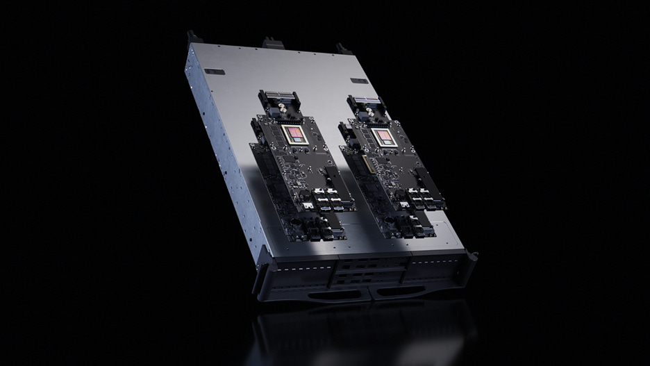
But is this really the case? If AI servers’ demand for DRAM is greater than for NAND, why did Jensen release a brand-new Memory Storage Platform at this week’s CES conference (see the figure below), which is equipped with four Bluefield 4 DPUs, each DPU supporting 150 TB of NAND capacity — this is essentially a NAND storage server tailor-made for NVIDIA’s AI server racks:

In today’s article, I will conduct a detailed calculation to estimate the memory demand of the “text-to-video” multimodal models, and at the same time answer the above DRAM vs. NAND question for readers.

In my previous article（From CNN (Convolutional Neural Network) to Transformer）, I mentioned that the Transformer has essentially become a general-purpose information processing framework. Because everything can be tokenized (for example, images can be split into patches), it can also implement multimodal interfaces (with images and text encoded into the same vector space). So next, on this basis, let me explain Sora’s underlying architecture, the Diffusion Transformer (DiT).

Before delving into DiT, let’s first introduce the Diffusion model. In order to understand how Diffusion models “generate” images, we must first understand how they “destroy” images.

We know the Second Law of Thermodynamics: in an isolated system, Entropy always increases monotonically over time until the system reaches thermodynamic equilibrium. Imagine dropping a drop of ink into a cup of clear water. At first, the ink molecules are highly concentrated; as time passes, the ink molecules gradually diffuse and eventually become evenly distributed throughout the entire cup of water - this is the forward process of diffusion models. However, in 1982, Brian Anderson proved a surprising theorem in Reverse-time diffusion equation models: for any diffusion process that satisfies certain conditions, there exists a reverse stochastic differential equation that can describe the reverse evolution of that process along the time axis.

Therefore, Diffusion models can be intuitively imagined as an AI version of the physical diffusion process described above: First, real samples are gradually corrupted by adding noise until they almost become Gaussian noise; Then, a neural network is trained to learn how to pull the noise back step by step. This “pulling back” direction is the gradient of the log density of the data distribution at each noise level. By denoising in many small steps along this direction, pure noise can be turned into a valid image or a segment of video.

Here, the backbone network of Diffusion models almost without exception initially chose the U-Net architecture (the U-shaped network at the bottom of the figure above, a type of CNN). The Diffusion Transformer, on the other hand, builds on Diffusion by borrowing the core ideas of the Vision Transformer (ViT): the Transformer architecture itself is universal and does not care whether the tokens come from text, audio, or images.

Source: Sora: A Review on Background, Technology, Limitations, and Opportunities of Large Vision Models

To facilitate the later calculation of storage requirements, I will briefly explain the core architecture of the Diffusion Transformer from a technical perspective here, which is built on three key components:

Variational Autoencoders (VAE): Specifically, DiT does not operate in the original Pixel Space. This is because if a Transformer is run directly on an image such as 512 × 512 × 3, the quadratic complexity of its self-attention mechanism would be computationally disastrous (N = 512 × 512). Therefore, as the first stage, in order to reduce computation, a VAE/ Autoencoder is first used to encode the image into a low-dimensional latent space, such as 64 × 64 × 4, allowing the diffusion process to operate in the latent space and greatly reducing computational cost.

Spacetime Latent Patches: DiT does not treat video as a sequence of independent frames; instead, it “patchifies” the video in latent space, creating “spacetime patches” or “tokens” that contain both spatial (2D) and temporal (Time) information. These tokens become the basic processing units of the model, analogous to tokens in LLMs. Moreover, because Transformers cannot directly process 2D grids, they require a 1D token sequence, so DiT adopts the ViT “patchify” strategy. It can divide a 64 × 64 × 4 latent representation into a series of non-overlapping patches. For example, using a 2 × 2 patch size (p = 2), we obtain (64/2) × (64/2) = 32 × 32 = 1024 patches. Each patch (for example, of size 2 × 2 × 4) is “flattened” and “embedded” into a fixed-dimensional token by a linear layer. Thus, a single image (its latent representation) is converted into a sequence containing 1024 tokens. As with ViT, the model adds “positional embeddings” to let the Transformer know the original 2D/ 3D position of each patch. After that, the latent-space features are cut into patches (for images) or tubelets (for videos, i.e., small blocks spanning time × space), linearly projected into a token sequence, and fed into the Transformer stack.

Diffusion Transformer Block: The self-attention mechanism of the Transformer enables it to capture ultra-long-range dependencies between spacetime patches, which is crucial for maintaining global consistency and coherence in videos. The time step and class labels are respectively converted into two conditioning vectors through their own embedding layers. Adaptive Layer Normalization (adaLN) injects these two conditioning vectors into the Transformer’s computation. adaLN can be understood as “reminding” the model in every Transformer block: “you are currently at time step 500 and are drawing a cat.”

So, to briefly summarize here, the principle by which DiT generates video is as follows: a gigantic Transformer that performs attention computation over tens of thousands of spacetime tokens, while simultaneously injecting multiple conditioning tokens such as text / image / cameo / timeline, continuously makes predictions during the diffusion process and gradually drives the “latent world” from Gaussian noise to converge toward a physically plausible spacetime trajectory.

By the way, on DiT, researchers also further validated the Scaling Law. They found that for any fixed-size DiT model, investing more training compute leads to improved image generation quality.

The above analysis is based on the publicly available Sora-1 architecture, and since OpenAI has not disclosed the network structure of Sora-2, we can only make inferences from OpenAI’s technical report and system card. Compared with Sora-1, Sora-2 adds audio and strengthens physics and controllability. OpenAI has emphasized that its core is still the DiT-based world simulation framework, and Sora-2 uses many examples to stress that “even failures must obey physics,” such as a basketball realistically bouncing off the backboard instead of teleporting into the hoop, or glass shattering in a more natural way when it falls to the ground. Therefore, OpenAI likely used larger-scale and cleaner video data, such as scenes with physical interactions including sports and dance, and may also have introduced physical or geometric regularization at the loss level, or further employed human or model-based evaluators during post-training to score outputs, in order to improve physical plausibility and character consistency. The audio head may be a shallow Diffusion network that listens to video latents to predict waveforms. Thus, Sora-2 is very likely built on top of Sora-1, with more compute and data invested, continuing to move forward along the Scaling Law trajectory.

Having introduced the basic architecture of the DiT model, I will next estimate the potential memory demand of the DiT model:

Substack now supports friends referral programme. If you enjoy my newsletter, it would mean the world to me if you could invite friends to subscribe and read with us. When you use the “Share” button or the “Refer a friend” link below, you’ll get credit for any new subscribers. Simply send the link in a text, email, or share it on social media with friends:

When more friends use your referral link to subscribe, you’ll receive special benefits:

- 5 referrals for a free 3-month compensation

- 10 referrals for a free half-year compensation

- 20 referrals for a free full-year compensation.